In the previous section, we saw the location of 'C' of some common objects. In this section we will see systems where particles are distributed in space
1. Consider a particle 'P' situated in space
• Let it be situated at a certain distance from the origin 'O' of the frame of reference
♦ x-axis is shown in red
♦ y-axis is shown in green
♦ z-axis is shown in blue
• This is shown in fig.7.42 (a) below:
2. The particle is shown as a yellow sphere
• It's mass is 0.5 kg
• We see that:
♦ It is not situated on the x-axis
♦ It is not situated on the y-axis
♦ It is not situated on the xy-plane
♦ It is situated in space
3. We know the method to specify the positions of such particles
• The method can be written in 5 steps:
(i) Drop a perpendicular from 'P' onto the xy-plane
• This is indicated by the blue line in fig.7.42(b) above
• Note that, the yellow sphere is a bit transparent. We see the blue line starting from the exact center of the sphere
(ii) Let P' be the foot of the perpendicular
• From P', draw a perpendicular onto the x-axis
• This is indicated by the green line
(iii) From P', draw a perpendicular onto the y-axis
• This is indicated by the red line
(iv) Let the length of the red line be xP = 2 m
• Let the length of the green line be yP = 3 m
• Let the length of the blue line be zP = 2 m
(v) Then the coordinates of P are (xP, yP, zP) = (2,3,2)
4. Consider another particle Q. It's mass is 0.75 kg. This is shown in fig.7.43(a) below:
• Q will have it's own red, green and blue lines
• Let the lengths of those lines be 1 m, 2 m, and 1 m respectively
• So the coordinates (xQ, yQ, zQ) will be (1,2,1)
5. So we have a system consisting of two particles P and Q
• We want the location of the 'C' of this system
6. In such cases, the 'C' lies at a point whose coordinates are (X,Y,Z)
• We already know the method to find 'X' and 'Y'
7. We can apply the same method to find 'Z'
• But to find 'Z', the method should be applied in the z-direction
• As usual, the method involves only 4 steps:
(i) Take the distances (from the xy-plane) for each particle
(ii) Apply the 'due weightage'
(iii) Find the average of those 'weighted distances'
(iv) This average is the 'Z'
8. So we can write a new equation:
Eq.7.3: $\mathbf\small{Z=\frac{\sum{m_iz_i} }{\sum{m_i}}}$
9. Now we can form the table:
 10. From the table, we get:
$\mathbf\small{\sum{m_i}=1.25}$
$\mathbf\small{\sum{m_ix_i}=1.75}$
$\mathbf\small{\sum{m_iy_i}=3}$
$\mathbf\small{\sum{m_iz_i}=1.75}$
• Thus we get:
$\mathbf\small{X=\frac{\sum{m_ix_i} }{\sum{m_i}}=\frac{1.75}{1.25}=1.4\, \text{m}}$
$\mathbf\small{Y=\frac{\sum{m_iy_i} }{\sum{m_i}}=\frac{3}{1.25}=2.4\, \text{m}}$
$\mathbf\small{Z=\frac{\sum{m_iz_i} }{\sum{m_i}}=\frac{1.75}{1.25}=1.4\, \text{m}}$
11. Using these coordinates, we can mark 'C'. This is shown as a small white sphere in fig.7.43(b) above
• We see that, 'C' has it's own red, green and blue lines
♦ The length of it's red line = X = 1.4 m
♦ The length of it's green line = Y = 2.4 m
♦ The length of it's blue line = Z = 1.4 m
• Also note that, the 'C' lies on the line joining P and Q
• In such 3-dimensional problems, another easier method can be used. Let us see the details of that method:
1. In fig.7.44(a) below, a vector is shown in magenta color
• It's tail end coincides with 'O'
• It's tip coincides with the center of 'P'
■ So it is the position vector of P
• We can denote it as $\mathbf\small{\vec{r}_P}$. (Details here)
2. Imagine that, a person wants to go from O to P
• He can take either one of the two paths given below:
Path 1:
• This path is along the $\mathbf\small{\vec{r}_P}$. It starts from O and ends at P
Path 2:
This path has 3 segments:
■ Segment 1:
• This segment starts from O
• The person travels a distance xP
♦ xP is the length of the red line
♦ So 'magnitude' of travel is xP
• Direction of travel for this segment is: 'along the x-axis'
• So the magnitude and direction of this travel can be represented in vector form as: $\mathbf\small{(x_P)\hat{i}}$
• At the end of this travel, the person is at the foot of the green line
■ Segment 2:
• This segment starts from the foot of the green line
• The person travels a distance yP
♦ yP is the length of the green line
♦ So 'magnitude' of travel is yP
• Direction of travel for this segment is: 'parallel to the y-axis'
• So the magnitude and direction of this travel can be represented in vector form as: $\mathbf\small{(y_P)\hat{j}}$
• At the end of this travel, the person is at the foot of the blue line
■ Segment 3:
• This segment starts from the foot of the blue line
• The person travels a distance zP
♦ zP is the length of the blue line
♦ So 'magnitude' of travel is zP
• Direction of travel for this segment is: 'parallel to the z-axis'
• So the magnitude and direction of this travel can be represented in vector form as: $\mathbf\small{(z_P)\hat{k}}$
• At the end of this travel, the person reaches the particle P
3. So we see 3 vectors in path 2. If we add those vectors, we will reach P
• That means:
Path 2 = $\mathbf\small{(x_P)\hat{i}+(y_P)\hat{j}+(z_P)\hat{k}}$
4. The initial and final points in both paths 1 and 2 are the same
• So we can write: Path 1 = Path 2
• That is: $\mathbf\small{\vec{r}_P=(x_P)\hat{i}+(y_P)\hat{j}+(z_P)\hat{k}}$
5. The above equality in (4) can be established based on fig.7.44(b) also:
(i) In fig.7.44(b), there are a total of 5 vectors:
Red, green, blue, yellow and magenta
(ii) We want to prove this:
Magenta = red + green + blue
(iii) Consider the following three vectors:
Red, green and yellow
• Applying triangle law of vector addition, we get:
yellow = red + green
(iv) Consider the following three vectors:
Yellow, blue and magenta
• Applying triangle law of vector addition, we get:
Magenta = yellow + blue
(v) Now we expand 'yellow' using the result in (iii). We get:
Magenta = red + green + blue
• This is the required result that we mentioned in (ii)
6. So it is proved beyond doubt. We can confidently write:
$\mathbf\small{\vec{r}_P=(x_P)\hat{i}+(y_P)\hat{j}+(z_P)\hat{k}}$
• In this equation,
♦ $\mathbf\small{\vec{r}_P}$ is the position vector
♦ xP, yP and zP are the coordinates of P
■ So we can write:
The following two items are closely related:
(i) position vector of a particle
(ii) The coordinates of that particle
1. Consider a particle 'P' situated in space
• Let it be situated at a certain distance from the origin 'O' of the frame of reference
♦ x-axis is shown in red
♦ y-axis is shown in green
♦ z-axis is shown in blue
• This is shown in fig.7.42 (a) below:
 |
| Fig.7.42 |
• It's mass is 0.5 kg
• We see that:
♦ It is not situated on the x-axis
♦ It is not situated on the y-axis
♦ It is not situated on the xy-plane
♦ It is situated in space
3. We know the method to specify the positions of such particles
• The method can be written in 5 steps:
(i) Drop a perpendicular from 'P' onto the xy-plane
• This is indicated by the blue line in fig.7.42(b) above
• Note that, the yellow sphere is a bit transparent. We see the blue line starting from the exact center of the sphere
(ii) Let P' be the foot of the perpendicular
• From P', draw a perpendicular onto the x-axis
• This is indicated by the green line
(iii) From P', draw a perpendicular onto the y-axis
• This is indicated by the red line
(iv) Let the length of the red line be xP = 2 m
• Let the length of the green line be yP = 3 m
• Let the length of the blue line be zP = 2 m
(v) Then the coordinates of P are (xP, yP, zP) = (2,3,2)
4. Consider another particle Q. It's mass is 0.75 kg. This is shown in fig.7.43(a) below:
 |
| Fig.7.43 |
• Let the lengths of those lines be 1 m, 2 m, and 1 m respectively
• So the coordinates (xQ, yQ, zQ) will be (1,2,1)
5. So we have a system consisting of two particles P and Q
• We want the location of the 'C' of this system
6. In such cases, the 'C' lies at a point whose coordinates are (X,Y,Z)
• We already know the method to find 'X' and 'Y'
7. We can apply the same method to find 'Z'
• But to find 'Z', the method should be applied in the z-direction
• As usual, the method involves only 4 steps:
(i) Take the distances (from the xy-plane) for each particle
(ii) Apply the 'due weightage'
(iii) Find the average of those 'weighted distances'
(iv) This average is the 'Z'
8. So we can write a new equation:
Eq.7.3: $\mathbf\small{Z=\frac{\sum{m_iz_i} }{\sum{m_i}}}$
9. Now we can form the table:

$\mathbf\small{\sum{m_i}=1.25}$
$\mathbf\small{\sum{m_ix_i}=1.75}$
$\mathbf\small{\sum{m_iy_i}=3}$
$\mathbf\small{\sum{m_iz_i}=1.75}$
• Thus we get:
$\mathbf\small{X=\frac{\sum{m_ix_i} }{\sum{m_i}}=\frac{1.75}{1.25}=1.4\, \text{m}}$
$\mathbf\small{Y=\frac{\sum{m_iy_i} }{\sum{m_i}}=\frac{3}{1.25}=2.4\, \text{m}}$
$\mathbf\small{Z=\frac{\sum{m_iz_i} }{\sum{m_i}}=\frac{1.75}{1.25}=1.4\, \text{m}}$
11. Using these coordinates, we can mark 'C'. This is shown as a small white sphere in fig.7.43(b) above
• We see that, 'C' has it's own red, green and blue lines
♦ The length of it's red line = X = 1.4 m
♦ The length of it's green line = Y = 2.4 m
♦ The length of it's blue line = Z = 1.4 m
• Also note that, the 'C' lies on the line joining P and Q
• Now we know the method to find 'C' of the particles distributed in 3 dimensional space
1. In fig.7.44(a) below, a vector is shown in magenta color
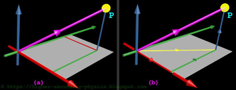 |
| Fig.7.44 |
• It's tip coincides with the center of 'P'
■ So it is the position vector of P
• We can denote it as $\mathbf\small{\vec{r}_P}$. (Details here)
2. Imagine that, a person wants to go from O to P
• He can take either one of the two paths given below:
Path 1:
• This path is along the $\mathbf\small{\vec{r}_P}$. It starts from O and ends at P
Path 2:
This path has 3 segments:
■ Segment 1:
• This segment starts from O
• The person travels a distance xP
♦ xP is the length of the red line
♦ So 'magnitude' of travel is xP
• Direction of travel for this segment is: 'along the x-axis'
• So the magnitude and direction of this travel can be represented in vector form as: $\mathbf\small{(x_P)\hat{i}}$
• At the end of this travel, the person is at the foot of the green line
■ Segment 2:
• This segment starts from the foot of the green line
• The person travels a distance yP
♦ yP is the length of the green line
♦ So 'magnitude' of travel is yP
• Direction of travel for this segment is: 'parallel to the y-axis'
• So the magnitude and direction of this travel can be represented in vector form as: $\mathbf\small{(y_P)\hat{j}}$
• At the end of this travel, the person is at the foot of the blue line
■ Segment 3:
• This segment starts from the foot of the blue line
• The person travels a distance zP
♦ zP is the length of the blue line
♦ So 'magnitude' of travel is zP
• Direction of travel for this segment is: 'parallel to the z-axis'
• So the magnitude and direction of this travel can be represented in vector form as: $\mathbf\small{(z_P)\hat{k}}$
• At the end of this travel, the person reaches the particle P
3. So we see 3 vectors in path 2. If we add those vectors, we will reach P
• That means:
Path 2 = $\mathbf\small{(x_P)\hat{i}+(y_P)\hat{j}+(z_P)\hat{k}}$
4. The initial and final points in both paths 1 and 2 are the same
• So we can write: Path 1 = Path 2
• That is: $\mathbf\small{\vec{r}_P=(x_P)\hat{i}+(y_P)\hat{j}+(z_P)\hat{k}}$
5. The above equality in (4) can be established based on fig.7.44(b) also:
(i) In fig.7.44(b), there are a total of 5 vectors:
Red, green, blue, yellow and magenta
(ii) We want to prove this:
Magenta = red + green + blue
(iii) Consider the following three vectors:
Red, green and yellow
• Applying triangle law of vector addition, we get:
yellow = red + green
(iv) Consider the following three vectors:
Yellow, blue and magenta
• Applying triangle law of vector addition, we get:
Magenta = yellow + blue
(v) Now we expand 'yellow' using the result in (iii). We get:
Magenta = red + green + blue
• This is the required result that we mentioned in (ii)
6. So it is proved beyond doubt. We can confidently write:
$\mathbf\small{\vec{r}_P=(x_P)\hat{i}+(y_P)\hat{j}+(z_P)\hat{k}}$
• In this equation,
♦ $\mathbf\small{\vec{r}_P}$ is the position vector
♦ xP, yP and zP are the coordinates of P
■ So we can write:
The following two items are closely related:
(i) position vector of a particle
(ii) The coordinates of that particle
7. Now, if 'Q' is another particle with coordinates (xQ,yQ,zQ), we can write:
$\mathbf\small{\vec{r}_Q=(x_Q)\hat{i}+(y_Q)\hat{j}+(z_Q)\hat{k}}$
8. Consider the system consisting of the two particles P and Q
• Let 'C' be the center of mass of the system
• The coordinates of 'C' are (X,Y,Z)
9. If we know those coordinates, we can easily write the position vector of 'C'
• Based on (6) above, we get: $\mathbf\small{\vec{r}_C=(X)\hat{i}+(Y)\hat{j}+(Z)\hat{k}}$
10. Now we expand X, Y and Z. We have:
• $\mathbf\small{X=\frac{m_p\,x_P+m_Q\,x_Q}{m_P+m_Q}=\frac{m_p\,x_P+m_Q\,x_Q}{M}}$
• $\mathbf\small{Y=\frac{m_p\,y_P+m_Q\,y_Q}{M}}$
• $\mathbf\small{Z=\frac{m_p\,z_P+m_Q\,z_Q}{M}}$
11. So the equation in (9) becomes:
$\mathbf\small{\vec{r}_C=\left[\frac{m_p\,x_P+m_Q\,x_Q}{M} \right]\hat{i}+\left[\frac{m_p\,y_P+m_Q\,y_Q}{M} \right]\hat{j}+\left[\frac{m_p\,z_P+m_Q\,z_Q}{M} \right]\hat{k}}$
$\mathbf\small{\Rightarrow \vec{r}_C=\frac{(m_P\,x_P)\hat{i}+(m_Q\,x_Q)\hat{i}+(m_P\,y_P)\hat{j}+(m_Q\,y_Q)\hat{j}+(m_P\,z_P)\hat{k}+(m_Q\,z_Q)\hat{k}}{M}}$
12. Now we rearrange the above equation by the two steps:
(i) Bringing the terms with mP together
(ii) Bringing the terms with mQ together
• We get:
$\mathbf\small{\vec{r}_C=\frac{[(m_P\,x_P)\hat{i}+(m_P\,y_P)\hat{j}+(m_P\,z_P)\hat{k}]+[(m_Q\,x_Q)\hat{i}+(m_Q\,y_Q)\hat{j}+(m_Q\,z_Q)\hat{k}]}{M}}$
• Taking mP and mQ outside, we get:
$\mathbf\small{\vec{r}_C=\frac{m_P[(x_P)\hat{i}+(y_P)\hat{j}+(z_P)\hat{k}]+m_Q[(x_Q)\hat{i}+(y_Q)\hat{j}+(z_Q)\hat{k}]}{M}}$
13. But:
♦ $\mathbf\small{(x_P)\hat{i}+(y_P)\hat{j}+(z_P)\hat{k}=\vec{r}_P}$
♦ $\mathbf\small{(x_Q)\hat{i}+(y_Q)\hat{j}+(z_Q)\hat{k}=\vec{r}_Q}$
• Thus (12) becomes:
$\mathbf\small{\vec{r}_C=\frac{m_P[\vec{r}_P]+m_Q[\vec{r}_Q]}{M}}$
14. This gives us an easy method to write the 'position vector of C'
• Let us check and see if we will get the same answer as before:
(i) The coordinates of P are (2,3,2)
• So $\mathbf\small{\vec{r}_P=2\hat{i}+3\hat{j}+2\hat{k}}$
• So $\mathbf\small{m_P\,\vec{r}_P=0.5(2\hat{i}+3\hat{j}+2\hat{k})=\hat{i}+1.5\hat{j}+\hat{k}}$
(ii) The coordinates of Q are (1,2,1)
• So $\mathbf\small{\vec{r}_Q=\hat{i}+2\hat{j}+\hat{k}}$
• So $\mathbf\small{m_Q\,\vec{r}_P=0.75(\hat{i}+2\hat{j}+\hat{k})=0.75\hat{i}+1.5\hat{j}+0.75\hat{k}}$
(iii) Thus the numerator in (13) becomes:
$\mathbf\small{(\hat{i}+1.5\hat{j}+\hat{k})+(0.75\hat{i}+1.5\hat{j}+0.75\hat{k})}$
$\mathbf\small{=(1.75\hat{i}+3.0\hat{j}+1.75\hat{k})}$
• The denominator M is the total mass = (mP + mQ) = (0.5+0.75) = 1.25 kg
(iv) Thus we get:
$\mathbf\small{\vec{r}_C=\frac{1.75\hat{i}+3.0\hat{j}+1.75\hat{k}}{1.25}=1.4\hat{i}+2.4\hat{j}+1.4\hat{k}}$
(v) So the coordinates of C are: (1.4,2.4,1.4)
• This is the same result that we obtained before
• P, Q, R, S, . . . are various particles in a system
• There are a total of 'n' particles in the system
♦ P is the first particle
♦ Q is the second particle
♦ R is the third particle . . . so on . . .
• Then:
♦ mP is the first mass
♦ mQ is the second mass
♦ mR is the third mass . . . so on . . .
16. We can write:
♦ m1 which is equal to mP is the first mass
♦ m2 which is equal to mQ is the second mass
♦ m3 which is equal to mR is the third mass . . . so on . . .
• Then:
♦ mi is the ith mass
♦ mn is the last mass
17. Also we can write:
♦ $\mathbf\small{\vec{r}_1}$ which is equal to $\mathbf\small{\vec{r}_P}$ is the first position vector
♦ $\mathbf\small{\vec{r}_2}$ which is equal to $\mathbf\small{\vec{r}_Q}$ is the second position vector
♦ $\mathbf\small{\vec{r}_3}$ which is equal to $\mathbf\small{\vec{r}_R}$ is the third position vector . . . so on . . .
• Then:
♦ $\mathbf\small{\vec{r}_i}$ is the ith position vector
♦ $\mathbf\small{\vec{r}_n}$ is the last position vector
18. So the equation in (13) becomes:
$\mathbf\small{\vec{r}_C=\frac{m_1\,\vec{r}_1+m_2\,\vec{r}_2\,+\,.\,.\,.\,+\,m_i\,\vec{r}_i+\,.\,.\,.\,+\,m_n\,\vec{r}_n}{m_1+m_2\,+\,.\,.\,.\,+\,m_i+\,.\,.\,.\,+\,m_n}}$
$\mathbf\small{\Rightarrow \vec{r}_C=\frac{m_1\,\vec{r}_1+m_2\,\vec{r}_2\,+\,.\,.\,.\,+\,m_i\,\vec{r}_i+\,.\,.\,.\,+\,m_n\,\vec{r}_n}{M}}$
19. Thus we get
Eq.7.4: $\mathbf\small{\vec{r}_C=\frac{\sum{} \,m_i\,\vec{r}_i}{M}}$
• This equation is applicable to 2- dimensional and 1-dimensional problems as well
• We will consider solved example 7.3. We will do it as a new solved example:
Solved example 7.7
Three particles P, Q and R are situated at the vertices of an equilateral triangle of side 0.5 m. Their masses are 100 g, 150 g and 200 g respectively. Find the location of the 'C' of this system of 3 particles
Solution:
1. We have three particles so situated in space that, they are at the vertices of an equilateral triangle
• For ease in calculations, we arrange the frame of reference in the following way:
♦ The plane of the triangle lies in the xy-plane
♦ One of the sides (say PQ), lies on the x-axis
♦ The left vertex (P) of that side coincides with O
• This arrangement is shown in fig.7.35 below:
2. Once this arrangement is fixed, we can easily write the coordinates of the bottom vertices
• The coordinates of P will be (0,0)
• The coordinates of Q will be (0.5,0)
• The x-coordinate of R will be 0.25
3. To find the y-coordinate of R, we use the following steps:
• Drop a perpendicular from R. This is shown in fig.b
• The foot of this perpendicular is R'
• In the right triangle PR'R, we have:
$\mathbf\small{\sin 60=\frac{RR'}{PR}=\frac{RR'}{0.5}}$
$\mathbf\small{\Rightarrow RR'=\sin 60 \times 0.5=0.433}$
So the y-coordinate of R is 0.433
4. Once we obtain the coordinates, we can write the position vectors:
(i) $\mathbf\small{\vec{r}_P=0\hat{i}+0\hat{j}}$
• This is a null vector
(ii) $\mathbf\small{\vec{r}_Q=0.5\hat{i}+0\hat{j}}$
(iii) $\mathbf\small{\vec{r}_R=0.25\hat{i}+0.433\hat{j}}$
5. We have: $\mathbf\small{\vec{r}_C=\frac{\sum{} \,m_i\,\vec{r}_i}{M}}$
• The numerator becomes: $\mathbf\small{0.1 \times 0+0.15 \times 0.5\hat{i}+0.2 \times 0.25\hat{i}+0.2 \times 0.433\hat{j}}$
= $\mathbf\small{0.125\hat{i}+0.0866\hat{j}}$
• The denominator is the total mass M = 0.450 kg
6. Thus we get: $\mathbf\small{\vec{r}_C=\frac{0.125\hat{i}+0.0866\hat{j}}{0.45}=0.278 \hat{i}+0.192 \hat{j}}$
7. So the coordinates of 'C' are: (0.278,0.192)
• This is the same result that we obtained earlier
• Note that, the unit vector $\mathbf\small{\hat{k}}$ does not come in the calculations because, this is a 2-dimensional problem
$\mathbf\small{\vec{r}_Q=(x_Q)\hat{i}+(y_Q)\hat{j}+(z_Q)\hat{k}}$
8. Consider the system consisting of the two particles P and Q
• Let 'C' be the center of mass of the system
• The coordinates of 'C' are (X,Y,Z)
9. If we know those coordinates, we can easily write the position vector of 'C'
• Based on (6) above, we get: $\mathbf\small{\vec{r}_C=(X)\hat{i}+(Y)\hat{j}+(Z)\hat{k}}$
10. Now we expand X, Y and Z. We have:
• $\mathbf\small{X=\frac{m_p\,x_P+m_Q\,x_Q}{m_P+m_Q}=\frac{m_p\,x_P+m_Q\,x_Q}{M}}$
• $\mathbf\small{Y=\frac{m_p\,y_P+m_Q\,y_Q}{M}}$
• $\mathbf\small{Z=\frac{m_p\,z_P+m_Q\,z_Q}{M}}$
11. So the equation in (9) becomes:
$\mathbf\small{\vec{r}_C=\left[\frac{m_p\,x_P+m_Q\,x_Q}{M} \right]\hat{i}+\left[\frac{m_p\,y_P+m_Q\,y_Q}{M} \right]\hat{j}+\left[\frac{m_p\,z_P+m_Q\,z_Q}{M} \right]\hat{k}}$
$\mathbf\small{\Rightarrow \vec{r}_C=\frac{(m_P\,x_P)\hat{i}+(m_Q\,x_Q)\hat{i}+(m_P\,y_P)\hat{j}+(m_Q\,y_Q)\hat{j}+(m_P\,z_P)\hat{k}+(m_Q\,z_Q)\hat{k}}{M}}$
12. Now we rearrange the above equation by the two steps:
(i) Bringing the terms with mP together
(ii) Bringing the terms with mQ together
• We get:
$\mathbf\small{\vec{r}_C=\frac{[(m_P\,x_P)\hat{i}+(m_P\,y_P)\hat{j}+(m_P\,z_P)\hat{k}]+[(m_Q\,x_Q)\hat{i}+(m_Q\,y_Q)\hat{j}+(m_Q\,z_Q)\hat{k}]}{M}}$
• Taking mP and mQ outside, we get:
$\mathbf\small{\vec{r}_C=\frac{m_P[(x_P)\hat{i}+(y_P)\hat{j}+(z_P)\hat{k}]+m_Q[(x_Q)\hat{i}+(y_Q)\hat{j}+(z_Q)\hat{k}]}{M}}$
13. But:
♦ $\mathbf\small{(x_P)\hat{i}+(y_P)\hat{j}+(z_P)\hat{k}=\vec{r}_P}$
♦ $\mathbf\small{(x_Q)\hat{i}+(y_Q)\hat{j}+(z_Q)\hat{k}=\vec{r}_Q}$
• Thus (12) becomes:
$\mathbf\small{\vec{r}_C=\frac{m_P[\vec{r}_P]+m_Q[\vec{r}_Q]}{M}}$
14. This gives us an easy method to write the 'position vector of C'
• Let us check and see if we will get the same answer as before:
(i) The coordinates of P are (2,3,2)
• So $\mathbf\small{\vec{r}_P=2\hat{i}+3\hat{j}+2\hat{k}}$
• So $\mathbf\small{m_P\,\vec{r}_P=0.5(2\hat{i}+3\hat{j}+2\hat{k})=\hat{i}+1.5\hat{j}+\hat{k}}$
(ii) The coordinates of Q are (1,2,1)
• So $\mathbf\small{\vec{r}_Q=\hat{i}+2\hat{j}+\hat{k}}$
• So $\mathbf\small{m_Q\,\vec{r}_P=0.75(\hat{i}+2\hat{j}+\hat{k})=0.75\hat{i}+1.5\hat{j}+0.75\hat{k}}$
(iii) Thus the numerator in (13) becomes:
$\mathbf\small{(\hat{i}+1.5\hat{j}+\hat{k})+(0.75\hat{i}+1.5\hat{j}+0.75\hat{k})}$
$\mathbf\small{=(1.75\hat{i}+3.0\hat{j}+1.75\hat{k})}$
• The denominator M is the total mass = (mP + mQ) = (0.5+0.75) = 1.25 kg
(iv) Thus we get:
$\mathbf\small{\vec{r}_C=\frac{1.75\hat{i}+3.0\hat{j}+1.75\hat{k}}{1.25}=1.4\hat{i}+2.4\hat{j}+1.4\hat{k}}$
(v) So the coordinates of C are: (1.4,2.4,1.4)
• This is the same result that we obtained before
15. We will generalize this method:
• There are a total of 'n' particles in the system
♦ P is the first particle
♦ Q is the second particle
♦ R is the third particle . . . so on . . .
• Then:
♦ mP is the first mass
♦ mQ is the second mass
♦ mR is the third mass . . . so on . . .
16. We can write:
♦ m1 which is equal to mP is the first mass
♦ m2 which is equal to mQ is the second mass
♦ m3 which is equal to mR is the third mass . . . so on . . .
• Then:
♦ mi is the ith mass
♦ mn is the last mass
17. Also we can write:
♦ $\mathbf\small{\vec{r}_1}$ which is equal to $\mathbf\small{\vec{r}_P}$ is the first position vector
♦ $\mathbf\small{\vec{r}_2}$ which is equal to $\mathbf\small{\vec{r}_Q}$ is the second position vector
♦ $\mathbf\small{\vec{r}_3}$ which is equal to $\mathbf\small{\vec{r}_R}$ is the third position vector . . . so on . . .
• Then:
♦ $\mathbf\small{\vec{r}_i}$ is the ith position vector
♦ $\mathbf\small{\vec{r}_n}$ is the last position vector
18. So the equation in (13) becomes:
$\mathbf\small{\vec{r}_C=\frac{m_1\,\vec{r}_1+m_2\,\vec{r}_2\,+\,.\,.\,.\,+\,m_i\,\vec{r}_i+\,.\,.\,.\,+\,m_n\,\vec{r}_n}{m_1+m_2\,+\,.\,.\,.\,+\,m_i+\,.\,.\,.\,+\,m_n}}$
$\mathbf\small{\Rightarrow \vec{r}_C=\frac{m_1\,\vec{r}_1+m_2\,\vec{r}_2\,+\,.\,.\,.\,+\,m_i\,\vec{r}_i+\,.\,.\,.\,+\,m_n\,\vec{r}_n}{M}}$
19. Thus we get
Eq.7.4: $\mathbf\small{\vec{r}_C=\frac{\sum{} \,m_i\,\vec{r}_i}{M}}$
• This equation is applicable to 2- dimensional and 1-dimensional problems as well
• Let us apply it to a two dimensional problem that we solved in the previous section
Solved example 7.7
Three particles P, Q and R are situated at the vertices of an equilateral triangle of side 0.5 m. Their masses are 100 g, 150 g and 200 g respectively. Find the location of the 'C' of this system of 3 particles
Solution:
1. We have three particles so situated in space that, they are at the vertices of an equilateral triangle
• For ease in calculations, we arrange the frame of reference in the following way:
♦ The plane of the triangle lies in the xy-plane
♦ One of the sides (say PQ), lies on the x-axis
♦ The left vertex (P) of that side coincides with O
• This arrangement is shown in fig.7.35 below:
 |
| Fig.7.35 |
• The coordinates of P will be (0,0)
• The coordinates of Q will be (0.5,0)
• The x-coordinate of R will be 0.25
3. To find the y-coordinate of R, we use the following steps:
• Drop a perpendicular from R. This is shown in fig.b
• The foot of this perpendicular is R'
• In the right triangle PR'R, we have:
$\mathbf\small{\sin 60=\frac{RR'}{PR}=\frac{RR'}{0.5}}$
$\mathbf\small{\Rightarrow RR'=\sin 60 \times 0.5=0.433}$
So the y-coordinate of R is 0.433
4. Once we obtain the coordinates, we can write the position vectors:
(i) $\mathbf\small{\vec{r}_P=0\hat{i}+0\hat{j}}$
• This is a null vector
(ii) $\mathbf\small{\vec{r}_Q=0.5\hat{i}+0\hat{j}}$
(iii) $\mathbf\small{\vec{r}_R=0.25\hat{i}+0.433\hat{j}}$
5. We have: $\mathbf\small{\vec{r}_C=\frac{\sum{} \,m_i\,\vec{r}_i}{M}}$
• The numerator becomes: $\mathbf\small{0.1 \times 0+0.15 \times 0.5\hat{i}+0.2 \times 0.25\hat{i}+0.2 \times 0.433\hat{j}}$
= $\mathbf\small{0.125\hat{i}+0.0866\hat{j}}$
• The denominator is the total mass M = 0.450 kg
6. Thus we get: $\mathbf\small{\vec{r}_C=\frac{0.125\hat{i}+0.0866\hat{j}}{0.45}=0.278 \hat{i}+0.192 \hat{j}}$
7. So the coordinates of 'C' are: (0.278,0.192)
• This is the same result that we obtained earlier
• Note that, the unit vector $\mathbf\small{\hat{k}}$ does not come in the calculations because, this is a 2-dimensional problem
So now we know how to find the location of the 'C' of any given system. In the next section, we will see the significance of 'C'


